

Modern-Day pKa: Generating a 3D Rendering of the Expanded Chemical Space in ADMET Predictor® 11
As we prepared for the unveiling of ADMET Predictor® 11, our AI cheminformatics platform, we stood on the edge of a dataset so immense it teetered on the brink of abstraction. Imagine 1,000 objects in front of you, now imagine 50,000! The idea was to visually represent the expanded chemical space, including new data from our pharma and agrochemical partners, in a way that not only showed its magnitude but also the diversity in the type of data now available to users. The 3D rendering could then be used in our videos, graphics and other marketing materials.
How do you create a 3D rendering of 50k chemicals with little to no knowledge of 3D? You ask a smart co-worker. 🙂
Picture this: you’re deep in the world of chemical structures, surrounded by a sea of data, and your task is to bring over 50,000 molecular structures to life with no prior 3D experience. A daunting challenge, right? That’s exactly where our very own #cheminformatics wizard, Robert Fraczkiewicz, found himself. Robert went on a wild ride, one where numbers transformed into vivid tangible forms. Grab your popcorn, folks, as we delve into Robert’s epic voyage from the world of molecules to the realm of polygons.
TLDR: It’s a colorful and emotion-packed journey that takes science communication to another dimension! Scroll to the end to see the final result.
Enter Robert Fraczkiewicz, Research Fellow, Cheminformatics, Simulations Plus, Inc.:
It’s good to step out of your comfort zone from time to time. ☺
I have 0.00001% knowledge and exactly zero experience in 3D graphics. All I know is that 3D surfaces are approximated by a mesh of polygons, but even that miniscule knowledge came in handy in what I recently had to do.
Scientists are supposed to be great communicators and present results of their research in concise and understandable manner. Yeah, right. In one of my recent projects I received a huge influx of new experimental data along with molecular structures of associated chemicals and faced a challenge of answering the following question:
How similar/different are the chemicals from different sources?
That’s not a problem if you compare, say, 10 molecular structures, but in this case I had over 50,000 of them! (Since a given compound may have more than one ionization site, the total number of measured ionization constants for 50k compounds was over 70k.) In addition, we were under a contractual obligation to keep molecular structures strictly confidential. Hmmm. Fortunately, long ago chemists developed a concept of an abstract “chemical space” – a multidimensional space occupied by an estimated 10^60 molecular structures with their similarity as a measure of distance. (For comparison, astrophysicists estimate that the observable universe contains “just” 10^80 atoms.)
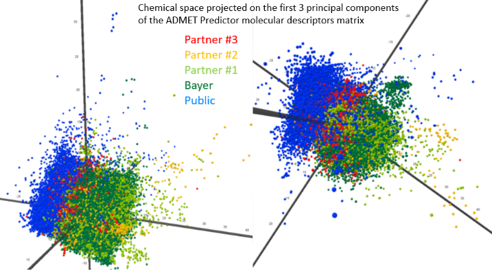
Thus, to answer the question posed above, should I present a table with 50,000 rows and 500 columns? Ouch! A picture is worth 1,000 words, so maybe show it as a set of points in 500-dimensional space? Ouch, humans can’t visualize 500 dimensions! Fortunately, mathematicians came to the rescue a long time ago – Principal Component Analysis allows one to project high dimensional spaces onto much more manageable 3D space. Miner3D in ADMET Predictor® made it easy and in a relatively short time I produced the image shown below – all 50,000+ chemicals colored by data source as points in 3D principal component space and that’s what I included in my PowerPoint presentation.
Victor, our Creative Lead, contacted me a short time afterwards with the following request: “What you have is just a static image. I want to create a video where the camera flies around and through this colorful cloud of points to show the scope of the new data. Can you export the 50,000 points as a 3D object?”
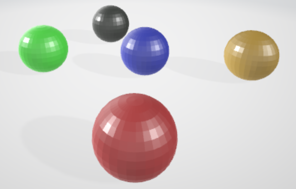
Cool! You mean 3D coordinates of each point? Sure! No, that’s not what Victor meant. “Each point is a sphere, right? I need 3D coordinates of all polygons that make all spheres so that I can render these in the 3D rendering software, Blender. Can Miner3D export as .OBJ?”
Ouch. No, it can’t. At this moment I felt like simply dismissing Victor with a, “No, can’t do” and move on, but the life of a scientist is all about solving problems, right? Thus, I accepted this out-of-my-comfort-zone challenge. Victor told me the .OBJ format opens up as a text file. “OK Victor, .OBJ is a human readable text? Send me a sample of, say, 5 spheres, each of different color.” He did.
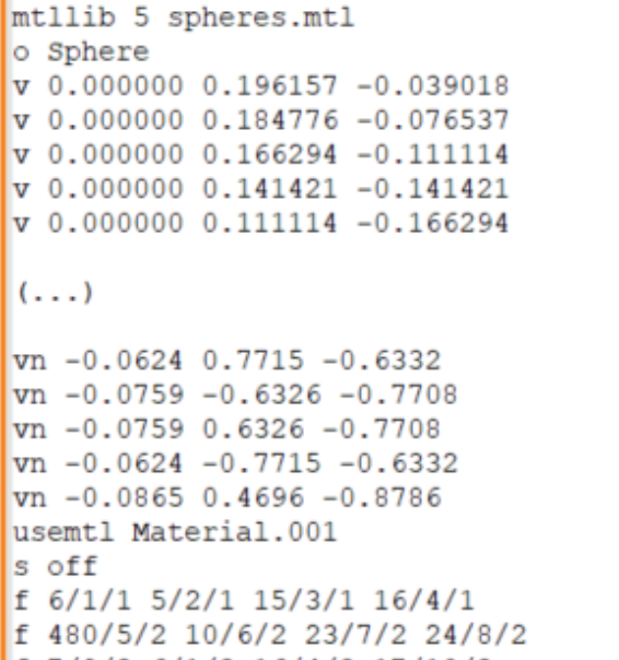
The associated “5spheres.obj” file opened in Notepad++, yay, but it was very far from being simple. Each sphere was encoded in over 2,000 lines of not so clear code/text! See for yourself:
Well, first things first – divide and conquer. I imported the “v” section into an old-fashioned Excel sheet and created a scatter plot of each pair of the X, Y, Z coordinates, here are two examples:
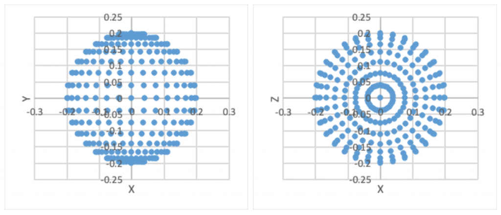
Indeed, “v’s” are vertices of polygons defining a sphere’s surface. OK, then “f’s” must be individual faces of the polyhedron approximating this sphere? But why four sets of integers? Time for an Internet search. Good, there exists a nice Wikipedia page describing the “Wavefront .OBJ format”. The “v’s” are geometric vertices, excellent, “vt’s” are texture coordinates, “vn’s” are vertex normal, and “f’s” are polygonal face elements.
So, having 50,000 sphere centers in 3D all I have to do is to generate polygonal vertices placed at a radius “r” for each sphere, then use indices of these vertices to define faces… Not so fast! A sphere is too complicated. What about something much simpler, like a regular tetrahedron? Four vertices and four faces? Good idea, but how to generate 3D coordinates of the four vertices having just the centroid? OK, it’s a little math problem and I like math. But the Wikipedia page on Tetrahedron spoils everything – it already has explicit formulas for each vertex. All right, I’ll take these without complaining. 😉 I take the first point and manually generate an .OBJ tetrahedron around it. Windows recognizes my .OBJ file as a “3D Object”. Hmm. I double-click it and bingo – it opens in an app called “3D Viewer”:

Cool, I didn’t even know such an app was native to Windows. As expected there is a blue tetrahedron that I can rotate in 3D and view from each side. Now all that remains to do is to generate ~49,999 more of these. Ouch. But I’m well versed in Excel and after a bit of hard work I had a “Tetrahedra.obj” file with 50,000 appropriately colored 3D objects, each at the right 3D position. Proudly smiling I sent it to Victor, but later that day he chilled me out: “I can’t use it.” Oh boy, why? “It opens fine in Blender, I can see all tetrahedra, but rendering of 50,000 objects takes extraordinarily long! There will be no animation from it.” Yeah, my file opens in 3D Viewer, too, but scaling and rotations are dog slow.
Bummer! Was all my hard work for nothing?
The same evening I’m in the shower thinking on how to solve this show stopping performance problem. 50k small objects… Each defined by four polygons… Hmm… Simple to draw one, but their number overwhelms rendering software… Hmm… The 5 spheres, each defined by 512 polygons… Hmm… And then and there an unusual thought strikes me: There is nothing in the .OBJ format that requires polygons to be connected! Wow. If I merge two tetrahedra into one object with 8 vertices and 8 faces will it still be rendered as two tetrahedra? I can’t wait to find out! I open my laptop before going to sleep. Yes! Two merged tetrahedra scale and rotate as one object. Three, four, ten? Yes and yes. Awesome! So instead of 50,000 3D objects I need just 5 – each composed of disconnected tetrahedra. In practice I find that 3D Viewer imposes a hard limit on the number of object’s polygons, at approximately 24,000 vertices, but I manage to define the whole set of 50,000 points as a set of just 10 3D objects. Phew. Each of these very quickly opens in 3D Viewer and rotations are lightning fast! Victor confirms the same happens in Blender – rendering performance is enhanced by orders of magnitude. Success!
After I received the final 3D models from Robert, I imported them into Blender to setup the lighting and cameras for the 3D scene.
I tracked the camera movement through the 3D molecules and around them to show the scope of the expansion.
The final render plus promotion videos below.